< Other courses
< Practical
Population genomic approaches
Preliminary analyses in population genomics - Tutorial - Last update: August 10, 2020
General context
Given the coronavirus disease 2019 (COVID-19) outbreak situation and the home learning situation, we have one additional day to work on population genetics analyses. The methods I want to introduce today are those that can be of interest to check the accuracy of a given dataset (including the reference genome used) and to carry out a preliminary analysis. All biological models can be relevant to introduce these additional (and very conventional) methods.
I decided to focus on the analysis of a handful of SARS-CoV2 genomes. I made this choice for several reasons (i) viral genomes are simple and have small genome sizes, thus allowing us to perform several different analyses using R on the same day, (ii) we will work on a plant species tomorrow and it was also important to work on a totally different kind of organism, (iii) we all receive a lot of information from journalists about the outbreak and the evolution of the virus. In the current context, I hypothesized that you could be interested by working on this topic and doing your own analyses.
Of course, the idea is not to perform detailed and publishable analyses (some papers are already published and a lot of excellent preprints are available), but rather to introduce a general course using these specific data. Our analyses will be only very preliminary and all our results need to be interpreted with caution. At the end of the pdf, you will find some additional links, including videos, if you are interested to learn more about the evolution of the SARS-CoV2 virus.
For legal reasons, I only used data that I am allowed to share with you, because these sequencing data are publicly available on the Sequence Read Archive (SRA). This data corresponds to a very limited proportion of the total number of sequences already sequenced available today all over the world.
Addditional notes: Given the situation with the home learning and considering your different backgrounds/computer skills, I decided to code all in R. Almost all steps can be done under a R environment (ideally under a Rstudio environment), but some additional R packages need to be loaded (and therefore, be installed). Depending of the R version you use, some problems during the installation are possible (and it is difficult to anticipate).
The main objective here is to understand the rationale, to read and write some lines of code, to perform the computations and interprete a little bit the output. If you want to do similar analyses on larger genomes (typically the genome you are interested in), I encourage you to write a similar code on another programing language and to only use R to make graphics using the newly generated output files. I can of course provide you some support.
This PDF file will help you to reproduce the commands. But you are highly encouraged to be curious and to edit the commands, to test some different parameters, etc. At the beginning of this course, you can copy/paste all the code, but it is important to read the code and try to understand the command, because toward the end of this PDF file, you will need to code more on your side.
For each function, if you want additional information, run
"?[NAME_OF_YOUR_FUNCTION]"
in the R console, e.g. "?plot". It will provide you a lot of information.
Step 1: Generate a multilocus alignment between 3 different SARS-CoV2 sequences using msa
Install the package "msa", if you have not already installed it:
install.packages("msa")
Load the package:
library("msa", dependencies = TRUE)
Define your working directory (in a linus/mac environment use forward slashes "/", in windows: use backward slashes "\""):
setwd("/home/thibaultleroy/covid19/")
Perform a whole genome alignment of 3 SARS-CoV2 genomes using ClustalW:
mySequence <- readDNAStringSet("
sequences_covid_SRA_030420.fasta.sed.completegenomes.3genomes")
Sys.time()
alignment <- msa(mySequence,method="ClustalW")
Sys.time()
How long did the alignment take?
Define a function to export an alignment in a fasta format
(to increase readibility I added the character "|" in the pdf (to show the loop in the code), but please do NOT write this pipe character in your code)
alignment2Fasta <- function(alignment, filename) {
| sink(filename)
| n <- length(rownames(alignment))
| for(i in seq(1, n)) {
| cat(paste0('>', rownames(alignment)[i]))
| cat('\n')
| the.sequence <- toString(unmasked(alignment)[[i]])
| cat(the.sequence)
| cat('\n')
| }
| sink(NULL)
|}
Export your alignment in a fasta "aligned.3SARSCOV2.fasta"
alignment2Fasta(alignment, 'aligned.3SARSCOV2.fasta')
Step 2: Generate a phylogenetic tree of 100 SARS-CoV2 genomes
Note: As you can imagine, the time needed to perform an alignment increases with the number of sequences to align, and this computational burden increases more than linearly. To speed up the process, I already provided you the file containing 100 fully aligned SARS-CoV2 genome sequences ("aligned.100genomes.v2.fasta"").
Read this alignment:
readalignment <- readDNAMultipleAlignment(
filepath = "aligned.100genomes.v2.fasta",format="fasta")
Install the package "seqinr" and "ape", if you have not already installed it:
install.packages("seqinr", dependencies = TRUE)
install.packages("ape", dependencies = TRUE)
Load the packages:
library("seqinr")
library("ape")
Read the alignment in the fasta format:
alignment <- msaConvert(readalignment, type="seqinr::alignment")
d <- dist.alignment(alignment2, "identity")
Generate a simple Neighbor-Joining tree following Saiton & Nei (1987):
sarscov2 <- nj(d)
plot(sarscov2, main="Phylogenetic tree of 100 SARS CoV2 sequences",
type="unrooted",cex=0.5)+ add.scale.bar()
A useful function "ape" function to reorder the internal structure of a tree (ladderize):
sarscov2_ladderize <-ladderize(sarscov2)
plot(sarscov2_ladderize, main="Phylogenetic tree of 100 SARS CoV2 sequences",
type="unrooted",cex=0.5)+ add.scale.bar()
You can display both trees at the same time using the par function "par(mfrow=c(LINES,COLUMNS)":
par(mfrow=c(1,2))
plot(sarscov2, main="Phylogenetic tree of 100 SARS CoV2 sequences",
type="unrooted",cex=0.5)+ add.scale.bar()
plot(sarscov2_ladderize, main="Phylogenetic tree of 100 SARS CoV2 sequences",
type="unrooted",cex=0.5)+ add.scale.bar()
It is possible to enhance readibility using some user-defined colors:
par(mfrow=c(1,1))
plot(sarscov2_ladderize, main="Phylogenetic tree of 100 SARS-CoV2 sequences",
type="cladogram",cex=0.5,
tip.color=ifelse(grepl("CHINA",sarscov2$tip.label),"darkblue",
ifelse(grepl("USA",sarscov2$tip.label),"red3",
ifelse(grepl("SPAIN",sarscov2$tip.label),"gold3",
ifelse(grepl("SWEDEN",sarscov2$tip.label),"orange",
ifelse(grepl("BRAZIL",sarscov2$tip.label),"darkorange3",
ifelse(grepl("PERU",sarscov2$tip.label),"darkorange4",
ifelse(grepl("INDIA",sarscov2$tip.label),"blue",
ifelse(grepl("AUSTRALIA",sarscov2$tip.label),"dodgerblue3",
ifelse(grepl("TAIWAN",sarscov2$tip.label),"midnightblue",
ifelse(grepl("NEPAL",sarscov2$tip.label),"darkslateblue",
ifelse(grepl("VIETNAM",sarscov2$tip.label),"dodgerblue4",
ifelse(grepl("PAKISTAN",sarscov2$tip.label),"darkslategray4","black")))))))))))),
edge.color="darkgrey")+ add.scale.bar(x=0.025,y=0,col="black",lcol="darkgrey")
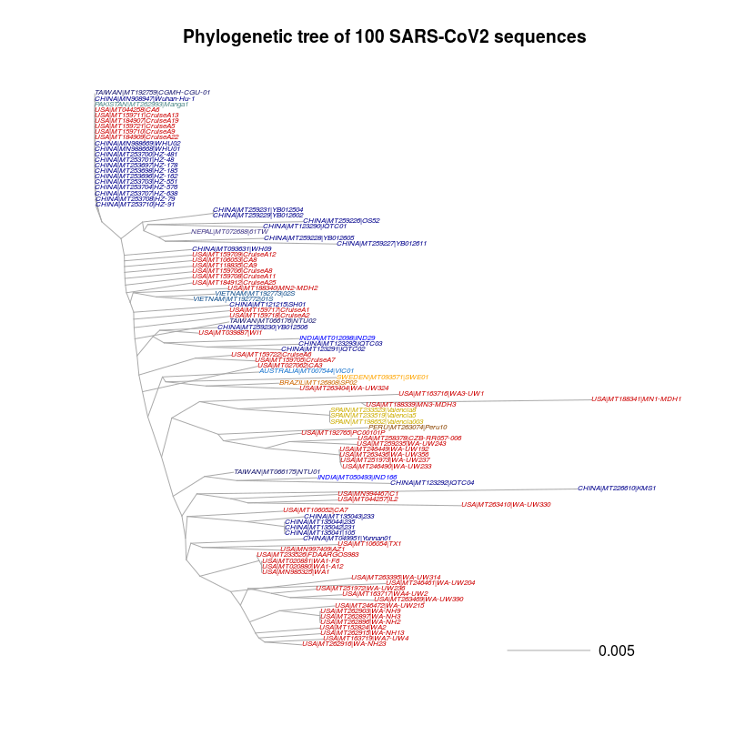
Note: you are free to change the commands. Here, the colors are set to be more or less in line with those used by Nextstrain (" https://nextstrain.org/ncov "). I strongly encourage you to spend some time to visit this website. Nextstrain is an excellent tool (the best to date and to my knowledge) for genetic data visualization of the SARS-CoV2 genomes. In particular, Nextstrain gives an explicit time information (i.e. when the strain was isolated, "TIME"), in addition of course to the sequence divergence. Combining the "clock" and the "time" options, Nextstrain can for example report you an estimate of the average number of substitions per year.
Step 3: Visualizing and editing multiple sequence alignments to generate a more reliable tree
Open your alignment on a sequence alignment software (you can download aliview, bioedit, etc...).
What can you observe on these alignments?
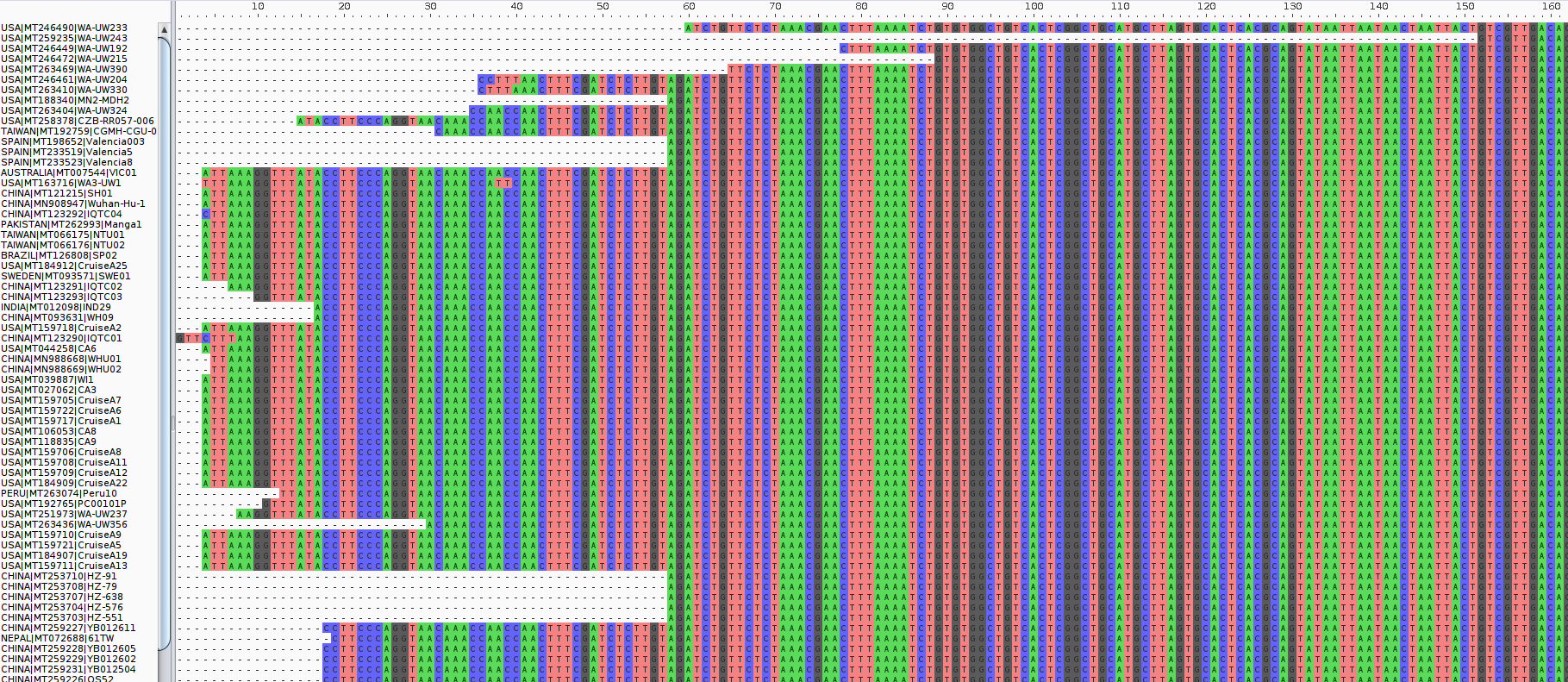
Try to remove the 200 first and the last 200 positions of the alignments. There are plenty of solutions to do this, more or less automatically, here an example of how to do this using a one line perl command (to be executed in your terminal):
perl -0076 -e 'while (<>) { chomp; my ($name, @parts) = split /\n/; my $seq = join "", @parts;
next unless defined $name && defined $seq; substr($seq, 0, 200, ""); print join "\n", ">".$name, "$seq\n" }'
INFILE.fasta | perl -0076 -e 'while (<>) { chomp; my ($name, @parts) = split /\n/; my $seq = join "", @parts;
next unless defined $name && defined $seq; substr($seq, -200, length($seq), ""); print join "\n", ">".$name,
l
"$seq\n" }'> OUTFILE.fasta
Open again your truncated alignement. Is it better?
If you can't generate this file this file is also available on moodle "aligned.100genomes.v2.200bases2EndsExcluded.fasta"
Redo the step 2 based on this new alignement. If possible, generate a figure with the two trees side by side and highlight the reference genome "MN908947" isolated from one of the first patients in Wuhan (Wu et al. 2020 Nature).
par(mfrow=c(1,2))
plot(sarscov2before, main="BEFORE CLEANING ALIGNMENTS",
type="cladogram",cex=0.5,
tip.color=ifelse(grepl("CHINA",sarscov2$tip.label),"darkblue",
ifelse(grepl("USA",sarscov2$tip.label),"red3",
ifelse(grepl("SPAIN",sarscov2$tip.label),"gold3",
ifelse(grepl("SWEDEN",sarscov2$tip.label),"orange",
ifelse(grepl("BRAZIL",sarscov2$tip.label),"darkorange3",
ifelse(grepl("PERU",sarscov2$tip.label),"darkorange4",
ifelse(grepl("INDIA",sarscov2$tip.label),"blue",
ifelse(grepl("AUSTRALIA",sarscov2$tip.label),"dodgerblue3",
ifelse(grepl("TAIWAN",sarscov2$tip.label),"midnightblue",
ifelse(grepl("NEPAL",sarscov2$tip.label),"darkslateblue",
ifelse(grepl("VIETNAM",sarscov2$tip.label),"dodgerblue4",
ifelse(grepl("PAKISTAN",sarscov2$tip.label),"darkslategray4","black")))))))))))),
edge.color="darkgrey",
font=ifelse(grepl("MN908947",sarscov2$tip.label),2,1))+
add.scale.bar(x=0.025,y=0,col="black",lcol="darkgrey")
plot(sarscov2, main="AFTER CLEANING ALIGNMENTS",
type="cladogram",cex=0.5,
tip.color=ifelse(grepl("CHINA",sarscov2$tip.label),"darkblue",
ifelse(grepl("USA",sarscov2$tip.label),"red3",
ifelse(grepl("SPAIN",sarscov2$tip.label),"gold3",
ifelse(grepl("SWEDEN",sarscov2$tip.label),"orange",
ifelse(grepl("BRAZIL",sarscov2$tip.label),"darkorange3",
ifelse(grepl("PERU",sarscov2$tip.label),"darkorange4",
ifelse(grepl("INDIA",sarscov2$tip.label),"blue",
ifelse(grepl("AUSTRALIA",sarscov2$tip.label),"dodgerblue3",
ifelse(grepl("TAIWAN",sarscov2$tip.label),"midnightblue",
ifelse(grepl("NEPAL",sarscov2$tip.label),"darkslateblue",
ifelse(grepl("VIETNAM",sarscov2$tip.label),"dodgerblue4",
ifelse(grepl("PAKISTAN",sarscov2$tip.label),"darkslategray4","black")))))))))))),
edge.color="darkgrey",
font=ifelse(grepl("MN908947",sarscov2$tip.label),2,1))+
add.scale.bar(x=0.025,y=0,col="black",lcol="darkgrey")
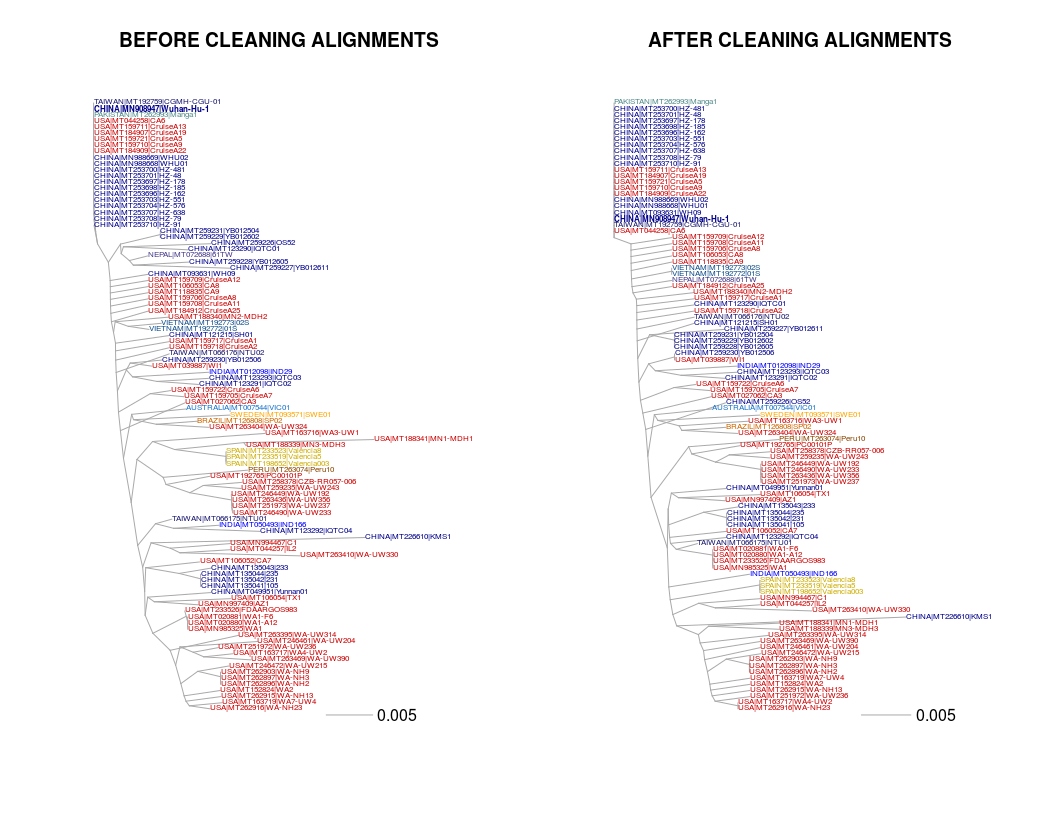
Note: In the case of the SARS-CoV2, it is quite easy to visualize the alignment (30kb genome only). But when we work on large genomes (through whole-genome alignments, or more likely read mapping), it is impossible to visually check these errors. But such errors are widespread (e.g. misidentification of one or several individuals, individuals with a lot of private alleles corresponding to sequence errors rather than true variants, etc...). Some fast methods can be really helpful to identify these weird individuals. In the following section, I introduce the importance of Principal Component Analyses.
Step 4: Principal Component Analyses
In the following section, we will focus on the importance of PCA for prelimary analyses of population genomics dataset. PCA are probably the most widely approaches used in this context. It allows to detect mislabeled samples in the dataset, but also to have a first look at the population structure.
As Ovidiu previously introduced, the VCF is the standard file format for storing genotype information. A simple convertion of your alignment in a vcf file can be done using snp-sites (in your terminal):
snp-sites -v aligned.100genomes.200bases2EndsExcluded.fasta
(If you have any issue with snp-sites, the file is also provided on moodle:
aligned.100genomes.v2.200bases2EndsExcluded.fasta.vcf).
Several R packages exist to perform a PCA in R (below I introduced two methods, in case you have any issue with the one of the packages).
Option 1 ("SNPRelate"):
Read your VCF file and perform the PCA:
library("SNPRelate")
vcf.fn<-"aligned.100genomes.v2.200bases2EndsExcluded.fasta.vcf"
snpgdsVCF2GDS(vcf.fn, "sarscov2.gds", method="biallelic.only")
genofile <- openfn.gds("sarscov2.gds")
out_pca1<-snpgdsPCA(genofile)
Generate a plot (e.g. for axes 1 and 2):
plot(out_pca1$eigenvect[,1],out_pca1$eigenvect[,2],
xlab=paste("PC 1 - ",round(out_pca1$varprop[1]*100,2),"% (option 1)"),
ylab=paste("PC 2 - ",round(out_pca1$varprop[2]*100,2),"%"),pch=20,cex=2,
col=ifelse(grepl("CHINA",out_pca1$sample.id),"darkblue",
ifelse(grepl("USA",out_pca1$sample.id),"red3",
ifelse(grepl("SPAIN",out_pca1$sample.id),"gold3",
ifelse(grepl("SWEDEN",out_pca1$sample.id),"orange",
ifelse(grepl("BRAZIL",out_pca1$sample.id),"darkorange3",
ifelse(grepl("PERU",out_pca1$sample.id),"darkorange4",
ifelse(grepl("INDIA",out_pca1$sample.id),"blue",
ifelse(grepl("AUSTRALIA",out_pca1$sample.id),"dodgerblue3",
ifelse(grepl("TAIWAN",out_pca1$sample.id),"midnightblue",
ifelse(grepl("NEPAL",out_pca1$sample.id),"darkslateblue",
ifelse(grepl("VIETNAM",out_pca1$sample.id),"dodgerblue4",
ifelse(grepl("PAKISTAN",out_pca1$sample.id),"darkslategray4","black")))))))))))))

Option 2 ("adegenet", using "vcfR"" to load the VCF"):
Read your VCF file and perform the PCA:
library("adegenet")
library(vcfR)
genofile <- vcfR2genlight(vcfRfile)
out_pca2 <- dudi.pca(genofile,cent=FALSE,scale=FALSE,scannf=FALSE,nf=5)
Compute the explained part of variance:
propvarexp=rbind(out_pca2$eig/sum(out_pca2$eig),cumsum(out_pca2$eig)/sum(out_pca2$eig))
Generate a plot (e.g. for axes 1 and 2):
plot(out_pca2$li[,1],out_pca2$li[,2],
xlab=paste("PC 1 - ",round(propvarexp[1,1]*100,2),"% (option2)"),
ylab=paste("PC 2 - ",round(propvarexp[1,2]*100,2),"%"),pch=20,cex=2,
col=ifelse(grepl("CHINA",rownames(out_pca2$tab)),"darkblue",
ifelse(grepl("USA",rownames(out_pca2$tab)),"red3",
ifelse(grepl("SPAIN",rownames(out_pca2$tab)),"gold3",
ifelse(grepl("SWEDEN",rownames(out_pca2$tab)),"orange",
ifelse(grepl("BRAZIL",rownames(out_pca2$tab)),"darkorange3",
ifelse(grepl("PERU",rownames(out_pca2$tab)),"darkorange4",
ifelse(grepl("INDIA",rownames(out_pca2$tab)),"blue",
ifelse(grepl("AUSTRALIA",rownames(out_pca2$tab)),"dodgerblue3",
ifelse(grepl("TAIWAN",rownames(out_pca2$tab)),"midnightblue",
ifelse(grepl("NEPAL",rownames(out_pca2$tab)),"darkslateblue",
ifelse(grepl("VIETNAM",rownames(out_pca2$tab)),"dodgerblue4",
ifelse(grepl("PAKISTAN",rownames(out_pca2$tab)),"darkslategray4","black")))))))))))))
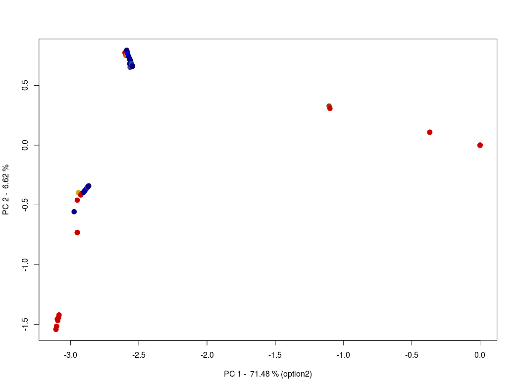
Using one of these two methods, generate a plot containing 4 panels (PC 1 & 2, PC 1 & 3, PC 1 & 4 and PC 2 & 3). If possible, continue to work on this small piece of code to automatically add an arrow pointing to the reference genome "MN908947" isolated from one of the first patients in Wuhan (Wu et al. 2020 Nature).
par(mfrow=c(2,2))
subsample=ccm_pca$eigenvect[grep("MN908947", ccm_pca$sample.id),]
plot(ccm_pca$eigenvect[,1],ccm_pca$eigenvect[,2],
xlab=paste("PC 1 - ",round(ccm_pca$varprop[1]*100,2),"% (option 1)"),
ylab=paste("PC 2 - ",round(ccm_pca$varprop[2]*100,2),"%"),
pch=20,cex=2,col=ifelse(grepl("CHINA",ccm_pca$sample.id),"darkblue",
ifelse(grepl("USA",ccm_pca$sample.id),"red3",
ifelse(grepl("SPAIN",ccm_pca$sample.id),"gold3",
ifelse(grepl("SWEDEN",ccm_pca$sample.id),"orange",
ifelse(grepl("BRAZIL",ccm_pca$sample.id),"darkorange3",
ifelse(grepl("PERU",ccm_pca$sample.id),"darkorange4",
ifelse(grepl("INDIA",ccm_pca$sample.id),"blue",
ifelse(grepl("AUSTRALIA",ccm_pca$sample.id),"dodgerblue3",
ifelse(grepl("TAIWAN",ccm_pca$sample.id),"midnightblue",
ifelse(grepl("NEPAL",ccm_pca$sample.id),"darkslateblue",
ifelse(grepl("VIETNAM",ccm_pca$sample.id),"dodgerblue4",
ifelse(grepl("PAKISTAN",ccm_pca$sample.id),"darkslategray4","black")))))))))))))
arrows(x=subsample[1],y1=subsample[2],x1=subsample[1],
y=subsample[2]-0.1*(max(ccm_pca$eigenvect[,2])-min(ccm_pca$eigenvect[,2])),
length=0.1,lwd=2,col="deeppink4")
plot(ccm_pca$eigenvect[,1],ccm_pca$eigenvect[,3],
xlab=paste("PC 1 - ",round(ccm_pca$varprop[1]*100,2),"% (option 1)"),
ylab=paste("PC 3 - ",round(ccm_pca$varprop[3]*100,2),"%"),
pch=20,cex=2,col=ifelse(grepl("CHINA",ccm_pca$sample.id),"darkblue",
ifelse(grepl("USA",ccm_pca$sample.id),"red3",
ifelse(grepl("SPAIN",ccm_pca$sample.id),"gold3",
ifelse(grepl("SWEDEN",ccm_pca$sample.id),"orange",
ifelse(grepl("BRAZIL",ccm_pca$sample.id),"darkorange3",
ifelse(grepl("PERU",ccm_pca$sample.id),"darkorange4",
ifelse(grepl("INDIA",ccm_pca$sample.id),"blue",
ifelse(grepl("AUSTRALIA",ccm_pca$sample.id),"dodgerblue3",
ifelse(grepl("TAIWAN",ccm_pca$sample.id),"midnightblue",
ifelse(grepl("NEPAL",ccm_pca$sample.id),"darkslateblue",
ifelse(grepl("VIETNAM",ccm_pca$sample.id),"dodgerblue4",
ifelse(grepl("PAKISTAN",ccm_pca$sample.id),"darkslategray4","black")))))))))))))
arrows(x=subsample[1],y1=subsample[3],x1=subsample[1],
y=subsample[3]-0.1*(max(ccm_pca$eigenvect[,3])-min(ccm_pca$eigenvect[,3])),
length=0.1,lwd=2,col="deeppink4")
plot(ccm_pca$eigenvect[,1],ccm_pca$eigenvect[,4],
xlab=paste("PC 1 - ",round(ccm_pca$varprop[1]*100,2),"% (option 1)"),
ylab=paste("PC 4 - ",round(ccm_pca$varprop[4]*100,2),"%"),
pch=20,cex=2,col=ifelse(grepl("CHINA",ccm_pca$sample.id),"darkblue",
ifelse(grepl("USA",ccm_pca$sample.id),"red3",
ifelse(grepl("SPAIN",ccm_pca$sample.id),"gold3",
ifelse(grepl("SWEDEN",ccm_pca$sample.id),"orange",
ifelse(grepl("BRAZIL",ccm_pca$sample.id),"darkorange3",
ifelse(grepl("PERU",ccm_pca$sample.id),"darkorange4",
ifelse(grepl("INDIA",ccm_pca$sample.id),"blue",
ifelse(grepl("AUSTRALIA",ccm_pca$sample.id),"dodgerblue3",
ifelse(grepl("TAIWAN",ccm_pca$sample.id),"midnightblue",
ifelse(grepl("NEPAL",ccm_pca$sample.id),"darkslateblue",
ifelse(grepl("VIETNAM",ccm_pca$sample.id),"dodgerblue4",
ifelse(grepl("PAKISTAN",ccm_pca$sample.id),"darkslategray4","black")))))))))))))
arrows(x=subsample[1],y1=subsample[4],x1=subsample[1],
y=subsample[4]-0.1*(max(ccm_pca$eigenvect[,4])-min(ccm_pca$eigenvect[,4])),
length=0.1,lwd=2,col="deeppink4")
plot(ccm_pca$eigenvect[,2],ccm_pca$eigenvect[,3],
xlab=paste("PC 2 - ",round(ccm_pca$varprop[2]*100,2),"% (option 1)"),
ylab=paste("PC 3 - ",round(ccm_pca$varprop[3]*100,2),"%"),
pch=20,cex=2,col=ifelse(grepl("CHINA",ccm_pca$sample.id),"darkblue",
ifelse(grepl("USA",ccm_pca$sample.id),"red3",
ifelse(grepl("SPAIN",ccm_pca$sample.id),"gold3",
ifelse(grepl("SWEDEN",ccm_pca$sample.id),"orange",
ifelse(grepl("BRAZIL",ccm_pca$sample.id),"darkorange3",
ifelse(grepl("PERU",ccm_pca$sample.id),"darkorange4",
ifelse(grepl("INDIA",ccm_pca$sample.id),"blue",
ifelse(grepl("AUSTRALIA",ccm_pca$sample.id),"dodgerblue3",
ifelse(grepl("TAIWAN",ccm_pca$sample.id),"midnightblue",
ifelse(grepl("NEPAL",ccm_pca$sample.id),"darkslateblue",
ifelse(grepl("VIETNAM",ccm_pca$sample.id),"dodgerblue4",
ifelse(grepl("PAKISTAN",ccm_pca$sample.id),"darkslategray4","black")))))))))))))
arrows(x=subsample[2],y1=subsample[3],x1=subsample[2],
y=subsample[3]-0.1*(max(ccm_pca$eigenvect[,3])-min(ccm_pca$eigenvect[,3])),
length=0.1,lwd=2,col="deeppink4")

Step 5: Compute base content over the reference genome (Wu et al. 2020 Nature)
In general, when we start to work on a new species. One of the first analysis we do is to look at the quality of the reference genome (assembly), in particular, the proportion of unknown nucleotide bases (N%) in the assembly. Here an example how to compute this proportion, after reading the data with seqinr.
Missing data or base composition over the whole genome
library("seqinr")
refgenome <- read.fasta(file = "reference_genome_wuhan-hu-1.fasta")
refgenomeseq <- refgenome[[1]]
N<- sum(lengths(regmatches(refgenomeseq, gregexpr("n", refgenomeseq))))
Ncontent=N/length(refgenomeseq)
print(paste("Ncontent:",Ncontent))
What do you conclude regarding the quality of the sequence based on the N%?
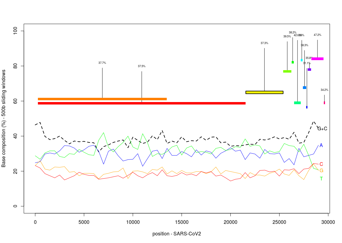
Modify this code to look the base content for each nucleobase (A,C,G,T for DNA, A,C,G,U for RNA). Given that the SARS-CoV2 is a single-stranded RNA virus, do you see something surprising? How can we explain this?
Base content using sliding windows along the whole genome
out=NULL
starts_win <- seq(1, length(refgenomeseq)-500, by = 500)
n <- length(starts_win)
|for (i in 1:n) {
| subsetwindow <- refgenomeseq[starts_win[i]:(starts_win[i]+499)]
| A<- sum(lengths(regmatches(subsetwindow, gregexpr("a", subsetwindow))))
| C<- sum(lengths(regmatches(subsetwindow, gregexpr("c", subsetwindow))))
| G<- sum(lengths(regmatches(subsetwindow, gregexpr("g", subsetwindow))))
| T<- sum(lengths(regmatches(subsetwindow, gregexpr("t", subsetwindow))))
| GCcontent <- sum(C,G)/sum(A,C,G,T,U)
| Acontent<- A/sum(A,C,G,T,U)
| Ccontent <- C/sum(A,C,G,T,U)
| Gcontent <- G/sum(A,C,G,T,U)
| Tcontent <- T/sum(A,C,G,T,U)
| out=rbind(out,cbind(starts_win[i],Acontent,Tcontent,Ccontent,Gcontent,GCcontent))
|}
out=as.data.frame(out)
colnames(out)=c("position","Acontent","Tcontent","Ccontent","Gcontent","GCcontent")
Generate a plot showing the variation of the base composition along the SARS-CoV2 genome:
plot(100*out$GCcontent~out$position,type="l",lwd=2,lty=2,ylim=c(0,100),xlab="position",
ylab="Base composition (%) - 500b sliding windows")+
lines(100*out$Acontent~out$position,type="l",col="blue")+
lines(100*out$Tcontent~out$position,type="l",col="green")+
lines(100*out$Gcontent~out$position,type="l",col="orange")+
lines(100*out$Ccontent~out$position,type="l",col="red")+
lines(100*out$Ucontent~out$position,type="l",col="darkgrey")+
text(x=tail(out$position,n=1)+300,y=tail(out$Acontent,n=1)*100,label="A",col="blue")+
text(x=tail(out$position,n=1)+300,y=tail(out$Tcontent,n=1)*100-5,label="T",col="green")+
text(x=tail(out$position,n=1)+300,y=tail(out$Gcontent,n=1)*100,label="G",col="orange")+
text(x=tail(out$position,n=1)+300,y=tail(out$Ccontent,n=1)*100,label="C",col="red")+
text(x=tail(out$position,n=1)+400,y=tail(out$GCcontent,n=1)*100,label="G+C",col="black")
Based on the provided gff (GCF_009858895.2_ASM985889v3_genomic.gff.mod.CDS) corresponding to the reference genome, try to write a piece of code providing the location of the different CDS on the previous plot, highlighting the gene YP_009724390, the gene coding for the Spike glyprotein, which is the protein initiating the infection by binding the human ACE2 receptor. Try also to indicate the per-gene GC content on the plot.
gff=read.table("GCF_009858895.2_ASM985889v3_genomic.gff.mod.CDS")
listcolor=rainbow(n=12)
for(i in 1:nrow(gff)){
| start=gff[i,4]
| end=gff[i,5]
| ypos=runif(1,min=55,max=85)
| rect(xleft=start,xright=end,ytop=ypos,ybottom=ypos-1.5,
| lwd=ifelse(grepl("YP_009724390", gff[i,9]),2,0),col=listcolor[i])
| yendline=runif(1,min=ypos,max=98)
| segments(x=start+(end-start)/2,y=ypos,x1=start+(end-start)/2,y1=yendline)
| geneseq=refgenomeseq[start:end]
| C<- sum(lengths(regmatches(geneseq, gregexpr("c",geneseq))))
| G<- sum(lengths(regmatches(geneseq, gregexpr("g",geneseq))))
| T<- sum(lengths(regmatches(geneseq, gregexpr("t",geneseq))))
| A<- sum(lengths(regmatches(geneseq, gregexpr("a",geneseq))))
| GCcontent <- sum(C,G)/sum(A,C,G,T)*100
| text(x=start+(end-start)/2,y=yendline+3,
| labels=paste(round(GCcontent,1),"%",sep=""),cex=0.55)
|}
Step 6: genetic variation along the genome
The distribution of the number of SNPs along the genome is also quite informative.
Using a new vcf file (aligned.100genomes.v2.200bases2EndsExcluded.fastacorr.vcf.clean, corrected to take into account some minor shifts in the genome positions) corresponding to the variants observed in our subset of 100 genomes, show the spatial distribution of the variants along the SARS-CoV2 genome.
Read the file and generate an histogram
vcfcor=read.table("aligned.100genomes.v2.200bases2EndsExcluded.fastacorr.vcf.clean")
hist(vcfcor$V2,breaks=29,col="lightgrey",border=FALSE,main="",xlab="Position - SARS-CoV2")
Add another layer to show the position of the SNPS, with different colors for transitions vs. transvertions
for(i in 1:nrow(vcfcor)){
| pos=vcfcor[i,2]
| baseref=vcfcor[i,4]
| basealt=vcfcor[i,5]
| segments(x=pos,y=-2,x1=pos,y1=-0.2,
col=ifelse(baseref=="A" && basealt=="G","red",
ifelse(baseref=="G" && basealt=="A","red",
ifelse(baseref=="C" && basealt=="T","red",
ifelse(baseref=="T" && basealt=="C","red","blue")))))
|}
text(x=29800,y=-0.5,labels="SNPs",cex=0.65,pos=4)
We can observe a clear hotspot of SNPs at one specific location of the genome. But the output seems a little bit different from those shown in the nextstrain webpage (https://nextstrain.org/ncov/global considering "Events" + "NT"). What do you think? You can of course reopen your alignment in your alignement viewer to reach a conclusion.
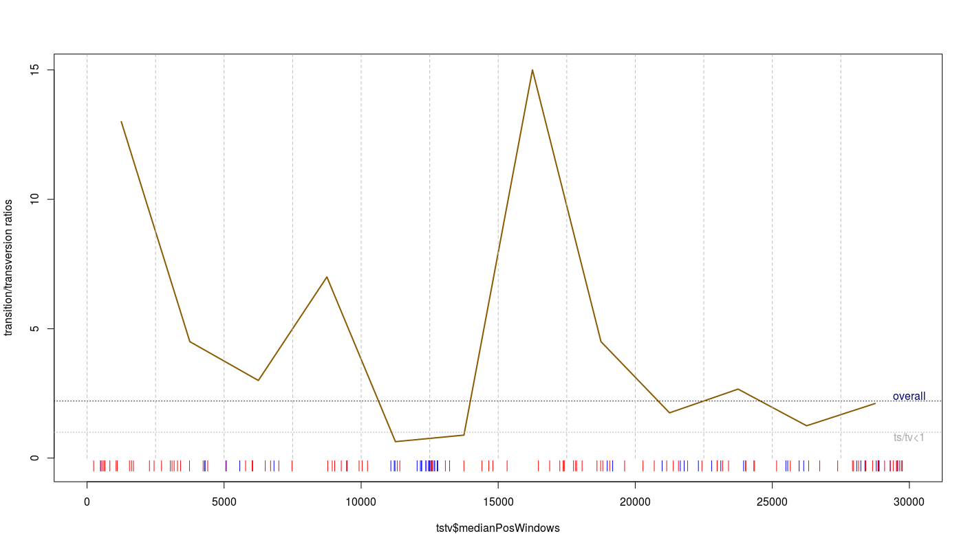
An additional conventional verification of a VCF file is to compute the ratio of transition vs. transversion (ts/tv)
Note: Mutation is a not a completely random process, transitions (C <=> T or G <=> A) are much more frequent than transversions (corresponding to all the other mutations possible). As a consequence, the ratio of transversion vs. transition is expected to be a good proxy of the quality of the calling (at least, when the number of mutations is non-limiting).
Compute the ts/tv ratio based on all variants detected over all SARS-CoV2 genomes we previously investigated:
A <- subset(vcfcor, V4=="A")
C <- subset(vcfcor, V4=="C")
G <- subset(vcfcor, V4=="G")
T <- subset(vcfcor, V4=="T")
transition1<- sum(lengths(regmatches(A$V5, gregexpr("G", A$V5))))
transition2<- sum(lengths(regmatches(G$V5, gregexpr("A", G$V5))))
transition3<- sum(lengths(regmatches(C$V5, gregexpr("T", C$V5))))
transition4<- sum(lengths(regmatches(T$V5, gregexpr("C", T$V5))))
totaltransitions=sum(transition1,transition2,transition3,transition4)
tstvratiowhole=totaltransitions/(nrow(vcfcor)-totaltransitions)
print(paste("ts/tv ratio:",tstvratiowhole))
Using this code, what is the value of ts/tv ratio?
Try to now create a piece of code to compute the ts/tv ratio over the genome using a sliding window approach (given the limited number of variants available, please use windows of >= 2.5kb in length). According to you, in which region the ts/tv ratio is informative about something bad with the data? Is it consistent with your previous investigations? As a consequence, what can you do to improve all our previous analyses?
tstv=NULL
lengthsequence=30001
starts_win <- seq(1, lengthsequence-2500, by = 2500)
n <- length(starts_win)
for (i in 1:n) {
| minregion=starts_win[i]
| maxregion=starts_win[i]+2499
| positionmedian=minregion+(maxregion-minregion)/2
| vcfcorregion <- subset(vcfcor, V2 >= minregion & V2 <= maxregion )
| A <- subset(vcfcorregion, V4=="A")
| C <- subset(vcfcorregion, V4=="C")
| G <- subset(vcfcorregion, V4=="G")
| T <- subset(vcfcorregion, V4=="T")
| transition1<- sum(lengths(regmatches(A$V5, gregexpr("G", A$V5))))
| transition2<- sum(lengths(regmatches(G$V5, gregexpr("A", G$V5))))
| transition3<- sum(lengths(regmatches(C$V5, gregexpr("T", C$V5))))
| transition4<- sum(lengths(regmatches(T$V5, gregexpr("C", T$V5))))
| totaltransitionsregion=sum(transition1,transition2,transition3,transition4)
| tstvratio=totaltransitionsregion/((nrow(vcfcorregion)-totaltransitionsregion))
| tstv=rbind(tstv,cbind(positionmedian,starts_win[i],starts_win[i]+2499,
totaltransitionsregion,nrow(vcfcorregion),tstvratio))
}
tstv=as.data.frame(tstv)
colnames(tstv)=c("medianPosWindows","startwindows","endwindows",
"transitions","totalSNP","tstvratio")
tstv[tstv == Inf] <- 15
plot(tstv$tstvratio~tstv$medianPosWindows,type="l",col="orange4",xlim=c(1,30000),
ylim=c(-0.3,15),lwd=2,ylab="transition/transversion ratios")+
abline(h=tstvratiowhole,lty=3,col="navyblue")+
abline(h=1,lty=3,col="darkgrey")+
text(x=30000,y=tstvratiowhole+0.2,label="overall",col="navyblue")+
text(x=30000,y=0.8,label="ts/tv<1",col="darkgrey")+
for(i in 1:nrow(tstv)){
| segments(x=tstv[i,2],x1=tstv[i,2],y=0,y1=16,col="grey",lty=2)
}
for(i in 1:nrow(vcfcor)){
| pos=vcfcor[i,2]
| baseref=vcfcor[i,4]
| basealt=vcfcor[i,5]
| segments(x=pos,y=-0.1,x1=pos,y1=-0.5,col=ifelse(baseref=="A" && basealt=="G","red",
ifelse(baseref=="G" && basealt=="A","red",ifelse(baseref=="C" && basealt=="T","red",
ifelse(baseref=="T" && basealt=="C","red","blue")))))
}
Interested to know more about the virus (including genetics & evolution)?
Interesting websites:
- NextStrain: https://nextstrain.org/ncov/
- ViralZone: https://viralzone.expasy.org/9056
Interesting webinars:
- Nicolas Bierne (CNRS): https://www.youtube.com/watch?v=OuiFUWko3yQ (starts at 23')
- Nextstrain Situation Report (e.g. 10 April: https://www.youtube.com/watch?v=_re0HORRLZ8 )
- Philippe Le Mercier (ViralZone): https://www.youtube.com/watch?v=h7oGqUHpA18
- Britt Glaunsinger (Berkeley): https://www.youtube.com/watch?v=8_bOhZd6ieM